A hierarchical triangular discrete global grid system on the icosahedron. Every parent cell is bit-for-bit the union of its four children, something neither hexagons nor pentagons can offer. A ~110 km cell has a 6-character address.
Launch the comparison demo
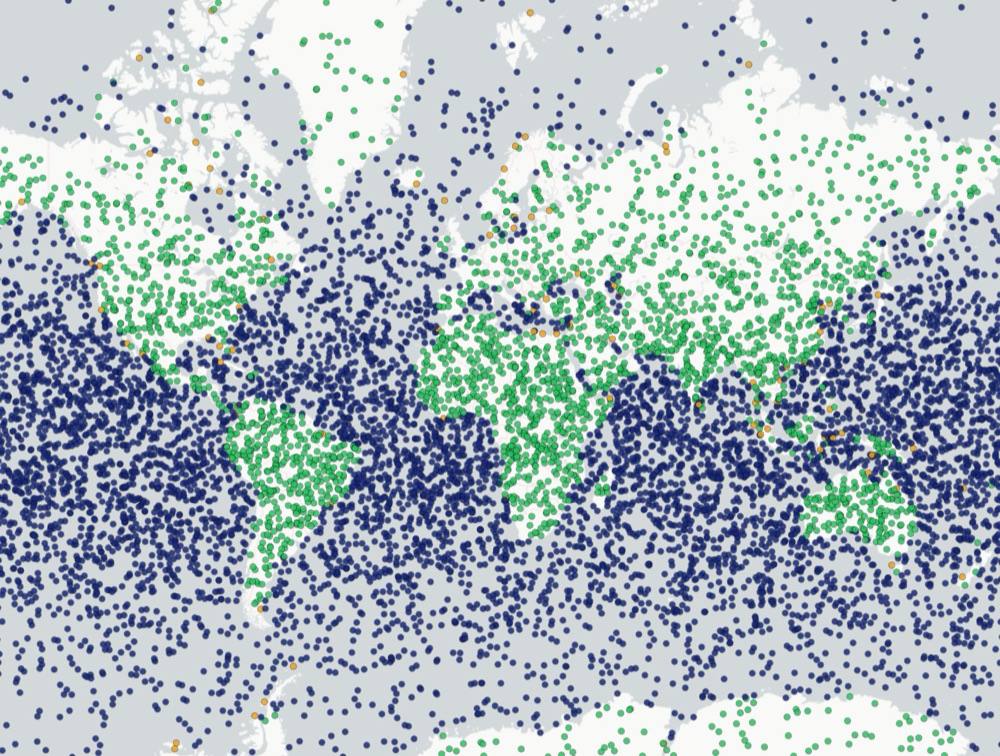
The first practical proof of concept of exact nesting: the level-10 land classification (~6.15M land-touching cells) collapses into 153,884 run-length intervals: a 182 KB dataset that answers "is this point on land?" in microseconds, fully offline, in Python and JavaScript, with a confidence value for every answer. Optional OSM refinement sharpens coastal answers to a near-exact polygon test.
Next on the roadmap is countrycheck, an offline country lookup using the same run-length approach with border-cell polygons.
One workload, four engines: classify 100,000 random points as land or sea against the same OSM land polygons. Trifold-based landcheck answered 3–30× faster than BigQuery, PostGIS and DuckDB Spatial in batch mode and 40–100× faster called one point at a time — true to the name, never less than a three-fold margin. The same gap should apply to similar point-classification problems.
Batch mode, median of 7 warm runs, Apple M5 Pro, June 2026. The SQL engines compute exact polygon containment; landcheck agrees with them on 99.5% of points from a far smaller dataset. Full benchmark with methodology and caveats →
Start from the icosahedron: 20 spherical triangles covering the Earth. Split every triangle into 4 by connecting the great-circle midpoints of its edges. Repeat. Each level halves the edge length and quadruples the cell count (aperture 4). Because children are built from the parent's own vertices plus edge midpoints, a parent cell is exactly the union of its children: aggregating data up the hierarchy or drilling down loses nothing and double-counts nothing.
| level | mean edge | mean area | cells (global) |
|---|---|---|---|
| 0 | 7,054 km | 25.5M km² | 20 |
| 3 | 882 km | 399k km² | 1,280 |
| 6 | 110 km | 6,226 km² | 81,920 |
| 9 | 13.8 km | 97 km² | 5.2M |
| 12 | 1.7 km | 1.5 km² | 336M |
| 15 | 215 m | 24 ha | 21.5B |
Parent = union of 4 children, verified to floating-point noise (10⁻¹⁹ of cell area). Lossless multi-resolution aggregation.
Both poles are lattice vertices: six meridian wedges meet at exactly ±90°. Antimeridian cells use continuous longitudes and are flagged. Classification uses polygon geometry.
Interior cells merge up the quadtree as far as they stay wholly on land; coastlines stay fine. 27,614 → 10,046 cells at level 6, identical 171.1M km² coverage.
One identity: compact base32 for humans, digit path for teaching, and a sortable uint64 for compute where a subtree is one contiguous range.
A cell is (face, path): one of 20 icosahedron faces plus a base-4 digit per
subdivision level (0,1,2 = corner children, 3 = central flipped
child). London at level 6:
| form | example | for | size |
|---|---|---|---|
| compact | TF6958 | humans, URLs, labels | 3 + ⌈2L/5⌉ chars |
| path | F15-102111 | teaching, debugging | 4 + L chars |
| addr64 | 8811996358392152070 | compute: sort, join, mask | 8 bytes |
Each triangle also carries two derived grouping keys. rhombus_id pairs
triangles exactly; rhombus_hilbert orders those pairs spatially within ten
base diamonds. hex_id provides six-triangle groups inside each icosahedron
face, with documented seam and vertex exceptions. These keys do not replace
addr64 or change the source geometry.
$ pip install -e . && trifold locate -0.1276 51.5072 6
TF6958
$ trifold show TF6958 # → path F15-102111 · edge ~117 km · area 5,864 km²
$ curl https://YOUR-WORKER.workers.dev/locate/-0.1276,51.5072?level=6
{"id":"TF6958","path":"F15-102111","addr64":"8811996358392152070","level":6}
Why base32 instead of digits 0–3? A digit string spends 8 bits per character to carry 2 bits. Crockford base32 packs 5 bits/char with no ambiguous I/L/O/U: same path bits at 40% of the length, URL-safe.
Trifold triangles vs A5 pentagons, H3 hexagons, S2 quads, rHEALPix, HTM (a related octahedral grid) and a plain lon/lat grid. Each layer uses the same land mask and styling. Toggle globe ↔ flat to compare the globe and Mercator projections; click any cell for its address and properties.
| T3 (this) | A5 | H3 | S2 | rHEALPix | HTM/QTM | |
|---|---|---|---|---|---|---|
| base solid | icosahedron | dodecahedron | icosahedron | cube | cube (HEALPix) | octahedron |
| cell shape | triangle | pentagon | hexagon (+12 pentagons) | quad | quad (+caps/darts) | triangle |
| aperture / nesting | 4, exact | 4, logical only | 7, approximate | 4, exact | 9, exact | 4, exact |
| equal area | ~±20%, smooth | exact per level | ~2× max/min | up to ~2× | near-exact | larger deformation |
| edge neighbours | 3 (+9 vertex) | 5 | 6 uniform | 4 | 4 | 3 (+vertex) |
| index | uint64, prefix=subtree | uint64, Hilbert | uint64 | uint64, Hilbert | string | quadtree string |
| ecosystem | this repository (2026) | introduced in 2025 | widely used | widely used | academic / OGC | astronomy |
Selection depends on the application. H3 provides uniform neighbour traversal and a mature ecosystem; S2 focuses on spatial indexing; rHEALPix and A5 provide equal-area cells. T3 focuses on exact hierarchical aggregation, variable-resolution tilings, and pipelines based on triangular geometry. Full analysis: technical reference.